This a series of step-by-step tutorials from the shapeXT manual. Each tutorial is designed to help you become familiar with shapeXT’s features and capabilities, from basic structure visualization to advanced analysis techniques.
For these tutorials, the crystal structure of NU-100 MOF is used as an example (COD ID: 1508131). The CIF is provided in the shapeXT examples directory.
You can open it via the menu (File > Examples > Tutorial_1_Manual_NU-100.cif), by dragging and dropping the file into the shapeXT window, or by using the File > Open dialog.
Getting Started with shapeXT
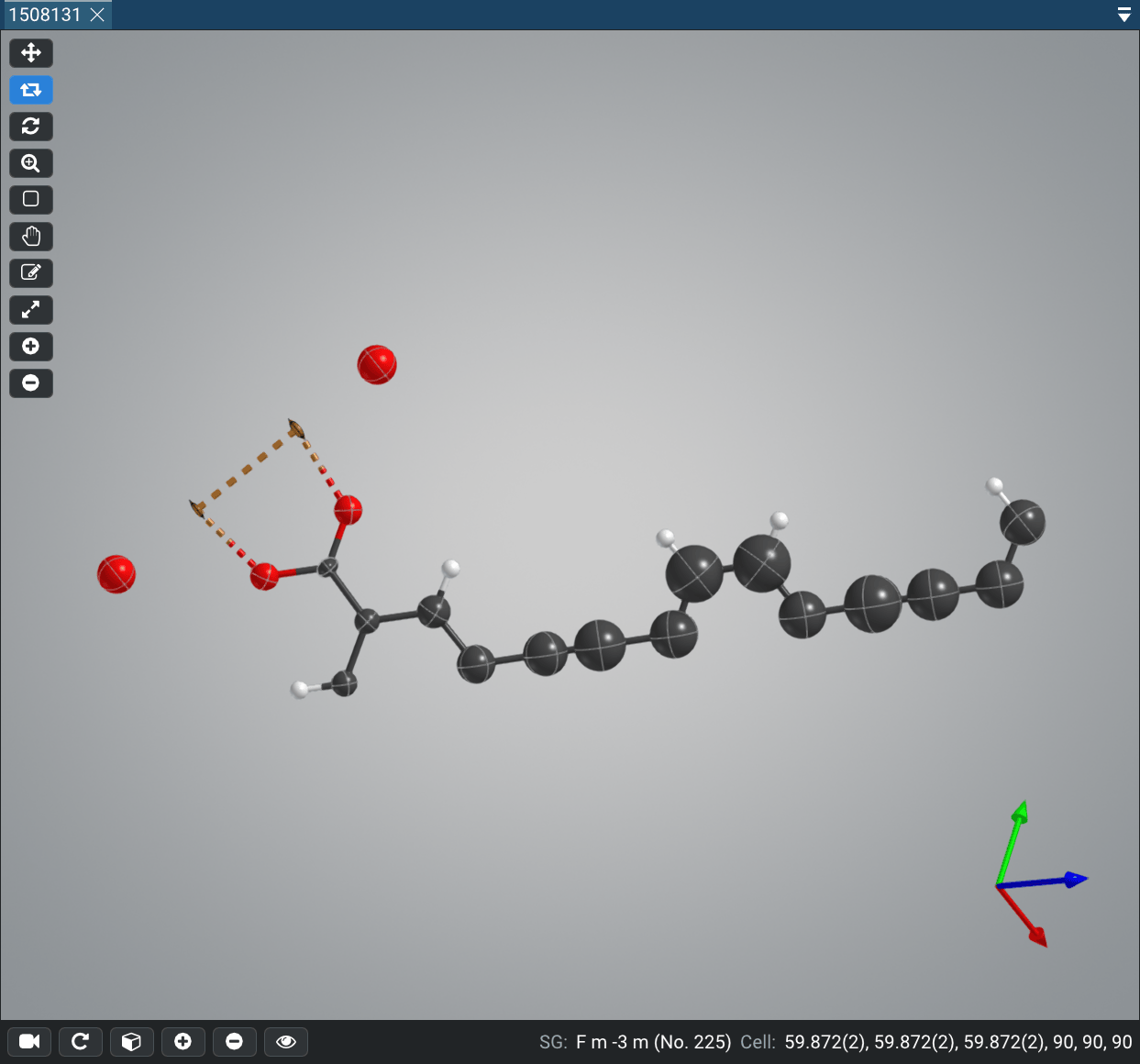
Once you have loaded Tutorial_1_Manual_NU-100.cif, you will get a view of the structure like in Figure 1.
For CIF structures, shapeXT generates by default only the asymmetric unit and tries to complete the fragments.
This is because the CIF format does not contain display information, e.g., which atoms have to be generated and rendered.
For shapeXT files (.sxt, .jsxt), the initial view is defined by the user and embedded into the file.
So the initial view of a shapeXT file is always the same as when the file was saved.
If you want to change the initial structure for your needs, go to Settings by pressing Ctrl+, or by clicking the gear icon in the bottom-left part of the sidebar.
At “Appearance > Default View” you can change the “Initial Structure” to various settings:
(a) Empty (No Atoms), (b) Asymmetric Unit, (c) Asymmetric Unit + Complete Fragments, (d) Unit Cell, (e) Unit Cell + Complete Fragments, (f) 2x2x2 Supercell, and (g) 2x2x2 Supercell + Complete Fragments.
Please note that you can also change other settings in this dialog like the default background color, the visibility of hydrogen atoms, and more.
After applying the changes, these initial settings will be used for all newly loaded structures.
Now, let’s move on with NU-100. The displayed initial structure is the asymmetric unit of the NU-100 structure with 26 atoms. This can be easily verified from the Navigator window which displays “Asymmetric Unit (26)” and “Atoms (26)”. Please also note that there is an unusually high number of detected molecules (97); we will come back to this later in the tutorial.
Bond Settings
If you look closely at the copper atoms of the paddlewheel core (Figure 1), there is a dashed bond between the two copper atoms, but no bond between the copper atoms and the apical oxygen atoms. If you hover over these dashed bonds, you will see data about the bond length and the bond type. The two equatorial Cu–O bonds have been identified as “dative” bonds, which is a special bond type in shapeXT. The dashed Cu–Cu bond is a special bond type called “metallophilic” which is used to indicate that the two atoms are part of a metal cluster. But since we are dealing with a Cu(II) paddlewheel core, we want to get rid of the dashed Cu–Cu bond and add the missing apical Cu–O bonds.
In a first step, shapeXT determines bonds automatically based on the atomic distances, covalent radii of the atoms, and a defined bond tolerance (default: 0.30 Å). A bond is created if the distance between two atoms is smaller than the sum of their covalent radii plus this defined bond tolerance. This classical bond detection algorithm is well-established and works for most structures. In addition, shapeXT utilizes a bond valence threshold approach to detect hydrogen bonds, dative bonds, vdW, and metallophilic interactions. Unfortunately, there is no single set of bond detection parameters that works for all structures, since there is a plethora of different structures with different bonding situations. That is why shapeXT provides a dialog so you can adjust the bond parameters for your structures.
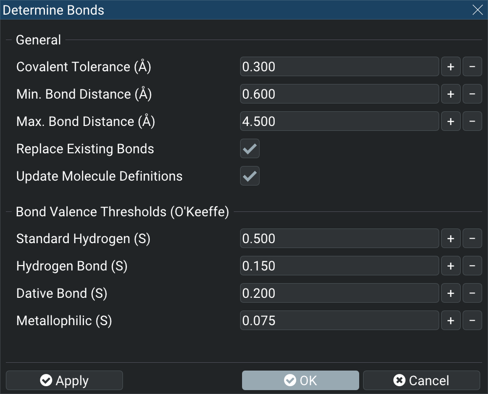
Click on “Build > Determine Bonds” to open the Determine Bonds dialog (Figure 2). This dialog window lets you adjust the bond detection parameters for the currently opened structure. If you want to adjust the bond detection parameters for all newly loaded structures, you can do this in the Settings dialog at “Chemistry > Bond Determination”.
To get rid of the dashed Cu–Cu metallophilic bond in NU-100, increase the bond valence threshold for metallophilic interactions to a higher value, e.g. 0.20. For the missing Cu–O dative bonds, decrease the bond valence threshold for dative interactions to a lower value, e.g. 0.10. Click on “Apply” to update the bond detection, move the dialog window to inspect the structure, and click on “OK” to close the dialog.
Expanding the Structure
After adjusting the bond parameters, note that the number of detected molecules in the “Navigator” has decreased from 97 to 1, which is the expected number for a 3D periodic coordination polymer without additional solvent molecules.
Since we have adjusted the bond situation, we can now expand the structure to visualize larger parts of the crystal structure.
In your structure view, select the plus icon (“Expand Atoms”) in the left toolbar of the structure view to change to the expansion mode.
This mode lets you expand individual atoms or fragments in your structure.
Click on the two copper atoms of the paddlewheel core to expand the coordination environment of the copper atoms.
To expand the whole structure, you can either press Ctrl+G or click on the “Expand Structure” icon in the bottom toolbar (plus icon) of the structure view.
If you want to undo the expansion, you can press Ctrl+Z or click on “Edit > Undo” in the menu.
To leave the expansion mode, click on the “Rotate Camera” mode or press R.
Selecting and Deleting Unwanted Atoms
Now, let us generate an image of the paddlewheel core of NU-100.
Since you have already expanded the structure, you may want to get rid of some of the generated atoms.
You can select objects by a selection rectangle by dragging the mouse while holding the right mouse button pressed.
The green selection rectangle indicates the selected area.
When you release the right mouse button, all objects within the selection rectangle will be selected.
You will notice the selection of objects by a change of color to a light green color.
When you repeat this process, the current selection will be replaced.
Therefore, if you want to add more objects to your current selection, hold the Shift key while selecting.
Once you have selected the unwanted atoms, you can delete them by pressing Del or by clicking on “Edit > Delete” in the menu.
If you have deleted too many atoms, you can undo the deletion by pressing Ctrl+Z or by clicking on “Edit > Undo” in the menu.
Adjusting the View
Once you have isolated the desired part of the paddlewheel core, you can adjust the view.
Press the X key to reset the zoom level.
Double tap the X key to reset the view (orientation and zoom).
You can also perform these adjustments via the “View” menu icon in the bottom toolbar of the structure view (“Reset Zoom” and “Reset View”).
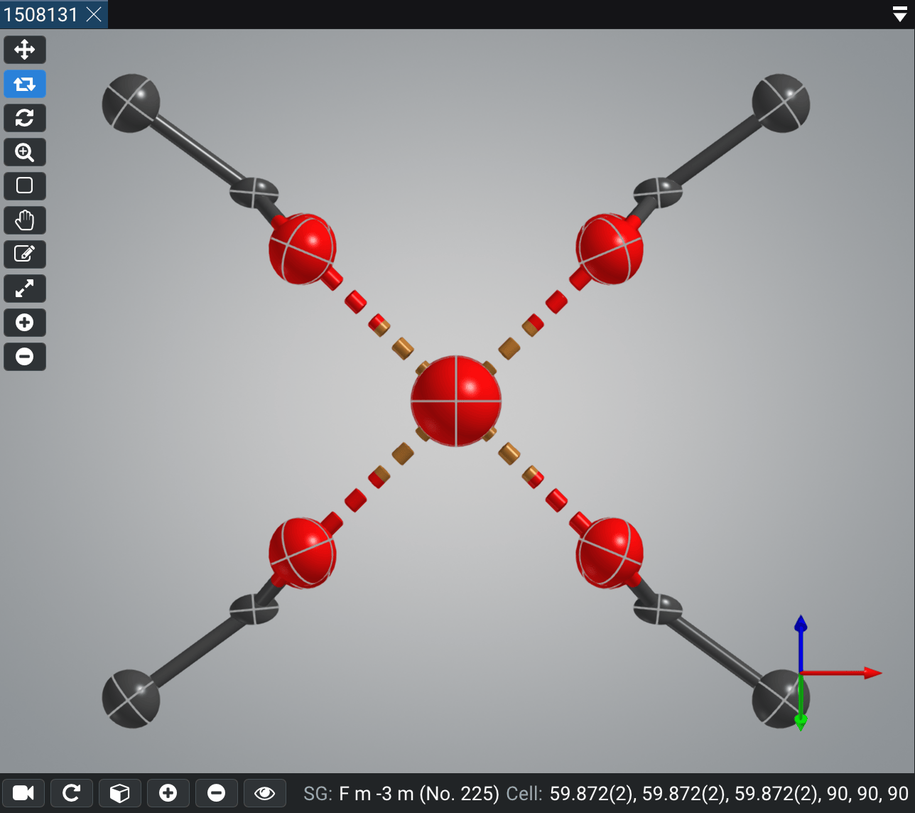
The result should look like Figure 3.
You can cycle quickly through the different views of the structure by pressing V or Shift+V.
In addition, you can always use the arrow keys to rotate the structure in small increments; hold the Shift key to rotate in larger increments.
To roll the structure, hold the Ctrl key while pressing the left or right arrow key.
Similarly, you can use the W-A-S-D keys to translate the structure in small increments, or press Shift+W or Shift+S to zoom in and out.
This way you can very quickly adjust the view of your structure without using the mouse.
Creating the first Image
Press Ctrl+Shift+C to copy the current structure to the clipboard as an image.
That’s it!
You can paste the image into your favorite image editor or directly into a document or presentation.
Now, you look at the image and think, “This is nice, but I want a black/white/transparent background.” For this task, you can click on the camera button on the sidebar to open the popup menu and below “Copy Image to Clipboard” select the desired background color: (a) “… with Black Background”, (b) “… with White Background”, or (c) “… with Transparent Background”. With these shortcuts, you can always copy your current structure view to the clipboard with the desired background color, e.g. transparent for presentations or white for publications.
Changing the background color of the structure view is also possible via a right click on an empty part of the structure view and selecting “Background > Presets”. You can also press F4 or Shift+F4 to cycle through the different background colors.
Lastly, you can also change the background color by selecting the General > Styles category in the Navigator and changing the background color(s) in the Inspector.
Image Rendering
If you want to instead save the image to a file directly, click on the camera button on the sidebar and choose “Export Image To File” and choose a desired background option. A dialog window will open where you can select the file format and the file name. This way, an image with the current dimensions of the structure view will be saved to a file, which is a fast and easy way to create images of your structures.
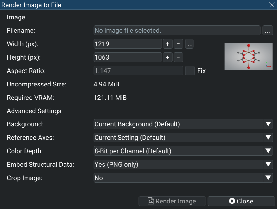
To have the full control over the image rendering, you can use the “Render Image To File” option in the camera menu (sidebar). This opens a dialog window (Figure 4) where you can set the image size, override the background color, change the color depth, hide reference axes, embed the structural data, or crop the image. Select a filename and click on “Render Image” to create the desired image file.
Continue?
Note that you can directly continue in the next tutorial of this series with your current structure.